Basic Tidyverse Concepts

(All Sections)

The `tidyverse` “Package”

Attach It

library(tidyverse)

── Attaching packages ─────────────────────────────────────── tidyverse 1.3.2 ──
✔ ggplot2 3.4.0      ✔ purrr   1.0.0 
✔ tibble  3.1.8      ✔ dplyr   1.0.10
✔ tidyr   1.2.1      ✔ stringr 1.5.0 
✔ readr   2.1.3      ✔ forcats 0.5.2 
── Conflicts ────────────────────────────────────────── tidyverse_conflicts() ──
✖ dplyr::filter() masks stats::filter()
✖ dplyr::lag()    masks stats::lag()

The Pipe Operator

The Pipe

%>% is from the magrittr package. (Some of this package is imported into the tidyverse.)

Usage:

# same as rep("hello", times = 4)
"hello" %>% rep(times = 4)

[1] "hello" "hello" "hello" "hello"

The Idea of the Pipe

The value returned by the first call becomes the first argument of the second call.

Another example:

# same as nrow(bcscr::m111survey)
bcscr::m111survey %>% nrow()

[1] 71

Piping to Another Argument

Use the . to pipe to an argument other than the first one:

# same as rep("hello", times = 4)
4 %>% rep("hello", times = .)

[1] "hello" "hello" "hello" "hello"

Another example:

# same as seq(1, 100, by = 4)[3]
seq(1, 100, by = 4) %>% .[3]

[1] 9

Practice

Rewrite the following call with the pipe operator, in three different ways:

seq(2, 22, by = 4)

[1]  2  6 10 14 18 22

Tibbles

Data Frames

What sort of thing is bcscr::m111survey?

class(bcscr::m111survey)

[1] "data.frame"

Yep, it’s a data frame.

Tibbles

Tibbles are similar to data frames. You can always turn a data frame into a tibble:

survey <- as_tibble(bcscr::m111survey)
class(survey)

[1] "tbl_df"     "tbl"        "data.frame"

Conveniences

The printout is compact:

survey

# A tibble: 71 × 12
   height ideal_ht sleep fastest weight_feel love_…¹ extra…² seat    GPA enoug…³
    <dbl>    <dbl> <dbl>   <int> <fct>       <fct>   <fct>   <fct> <dbl> <fct>  
 1   76         78   9.5     119 1_underwei… no      yes     1_fr…  3.56 no     
 2   74         76   7       110 2_about_ri… no      yes     2_mi…  2.5  no     
 3   64         NA   9        85 2_about_ri… no      no      2_mi…  3.8  no     
 4   62         65   7       100 1_underwei… no      no      1_fr…  3.5  no     
 5   72         72   8        95 1_underwei… no      yes     3_ba…  3.2  no     
 6   70.8       NA  10       100 3_overweig… no      no      1_fr…  3.1  yes    
 7   70         72   4        85 2_about_ri… no      yes     1_fr…  3.68 no     
 8   79         76   6       160 2_about_ri… no      yes     3_ba…  2.7  yes    
 9   59         61   7        90 2_about_ri… no      yes     3_ba…  2.8  no     
10   67         67   7        90 3_overweig… no      no      2_mi… NA    yes    
# … with 61 more rows, 2 more variables: sex <fct>, diff.ideal.act. <dbl>, and
#   abbreviated variable names ¹love_first, ²extra_life, ³enough_Sleep

This is an advantage when you are dealing with large amount of data.

Subsetting with dplyr

The dplyr package is part of the tidyverse. It contains function to manipulate data sets.

Pick Out Rows With `filter()`

survey %>%
  filter((sex == "male" & height > 70) | (sex =="female" & height < 55))

# A tibble: 22 × 12
   height ideal_ht sleep fastest weight_feel love_…¹ extra…² seat    GPA enoug…³
    <dbl>    <dbl> <dbl>   <int> <fct>       <fct>   <fct>   <fct> <dbl> <fct>  
 1   76         78   9.5     119 1_underwei… no      yes     1_fr…  3.56 no     
 2   74         76   7       110 2_about_ri… no      yes     2_mi…  2.5  no     
 3   72         72   8        95 1_underwei… no      yes     3_ba…  3.2  no     
 4   70.8       NA  10       100 3_overweig… no      no      1_fr…  3.1  yes    
 5   79         76   6       160 2_about_ri… no      yes     3_ba…  2.7  yes    
 6   73         77   6       110 2_about_ri… yes     yes     3_ba…  3.5  no     
 7   73         75   8       120 2_about_ri… no      yes     2_mi…  3.55 yes    
 8   54         54   4       130 3_overweig… yes     yes     1_fr…  3.41 no     
 9   74         75   5       119 2_about_ri… yes     yes     1_fr…  3.7  no     
10   72         90   9       125 3_overweig… no      yes     3_ba…  2.2  no     
# … with 12 more rows, 2 more variables: sex <fct>, diff.ideal.act. <dbl>, and
#   abbreviated variable names ¹love_first, ²extra_life, ³enough_Sleep

Pick Out Columns With `select()`

survey %>%
  select(sex, height, fastest)

# A tibble: 71 × 3
   sex    height fastest
   <fct>   <dbl>   <int>
 1 male     76       119
 2 male     74       110
 3 female   64        85
 4 female   62       100
 5 male     72        95
 6 male     70.8     100
 7 male     70        85
 8 male     79       160
 9 female   59        90
10 female   67        90
# … with 61 more rows

Chaining

filter() and select() are examples of data verbs: they operate on data tables.

A data verb:

takes a data table (data frame, tibble, etc.) as its first argument;
returns a data table.

Hence they may be composed easily.

Example of Chaining

survey %>% 
  filter((sex == "male" & height > 70) | (sex =="female" & height < 55)) %>% 
  select(sex, height, fastest)

# A tibble: 22 × 3
   sex    height fastest
   <fct>   <dbl>   <int>
 1 male     76       119
 2 male     74       110
 3 male     72        95
 4 male     70.8     100
 5 male     79       160
 6 male     73       110
 7 male     73       120
 8 female   54       130
 9 male     74       119
10 male     72       125
# … with 12 more rows

Leaving Columns Out

Put - signs in front of the columns you don’t want:

survey %>% 
  select(-ideal_ht, -love_first)

# A tibble: 71 × 10
   height sleep fastest weight_feel   extra_…¹ seat    GPA enoug…² sex   diff.…³
    <dbl> <dbl>   <int> <fct>         <fct>    <fct> <dbl> <fct>   <fct>   <dbl>
 1   76     9.5     119 1_underweight yes      1_fr…  3.56 no      male        2
 2   74     7       110 2_about_right yes      2_mi…  2.5  no      male        2
 3   64     9        85 2_about_right no       2_mi…  3.8  no      fema…      NA
 4   62     7       100 1_underweight no       1_fr…  3.5  no      fema…       3
 5   72     8        95 1_underweight yes      3_ba…  3.2  no      male        0
 6   70.8  10       100 3_overweight  no       1_fr…  3.1  yes     male       NA
 7   70     4        85 2_about_right yes      1_fr…  3.68 no      male        2
 8   79     6       160 2_about_right yes      3_ba…  2.7  yes     male       -3
 9   59     7        90 2_about_right yes      3_ba…  2.8  no      fema…       2
10   67     7        90 3_overweight  no       2_mi… NA    yes     fema…       0
# … with 61 more rows, and abbreviated variable names ¹extra_life,
#   ²enough_Sleep, ³diff.ideal.act.

Transforming Variables With `mutate()`

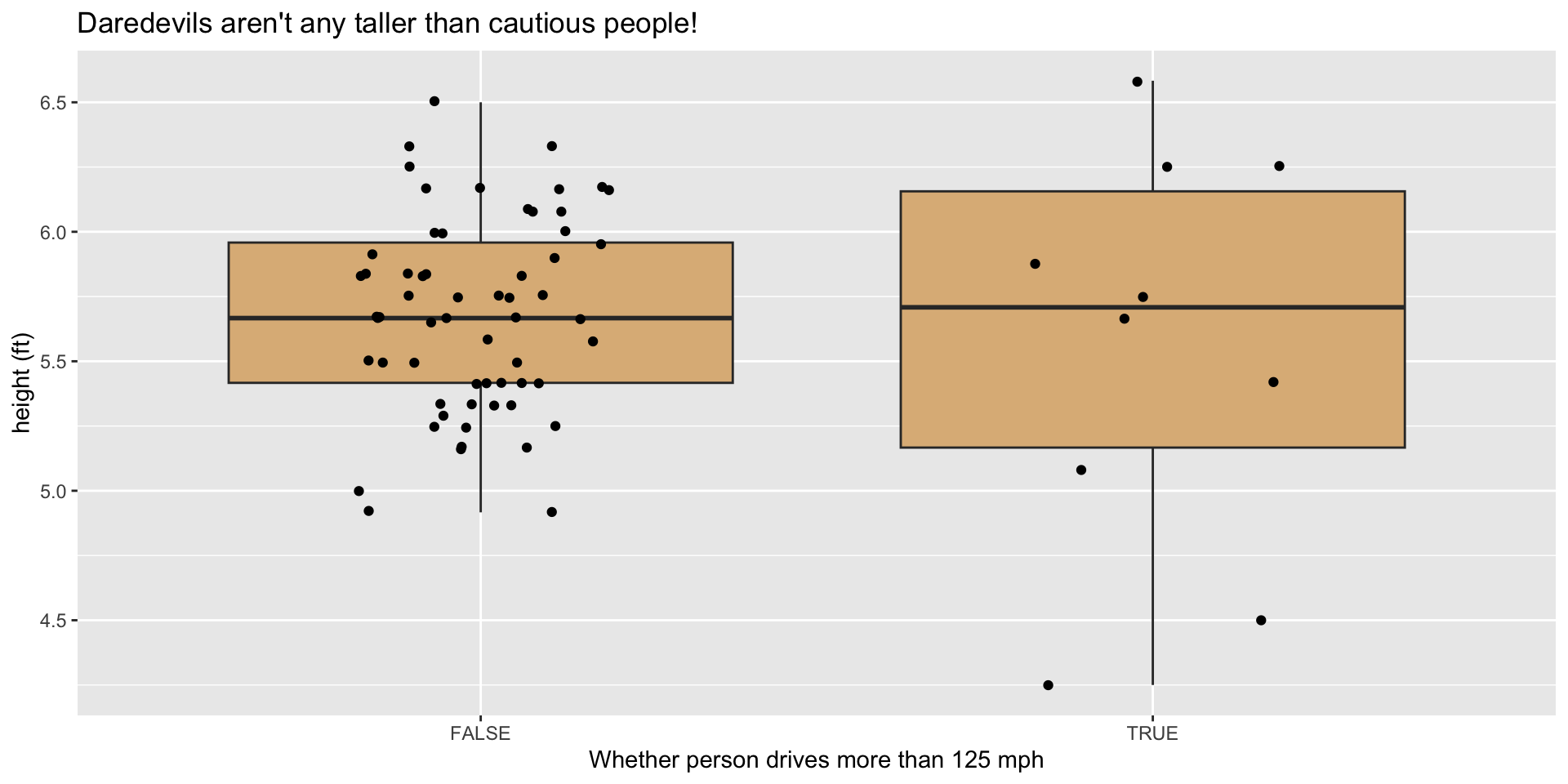
Classify Drivers

You’re a Daredevil if you go more than 125 mph:

survey %>% 
  mutate(dareDevil = fastest > 125) %>%
  select(sex, fastest, dareDevil)

# A tibble: 71 × 3
   sex    fastest dareDevil
   <fct>    <int> <lgl>    
 1 male       119 FALSE    
 2 male       110 FALSE    
 3 female      85 FALSE    
 4 female     100 FALSE    
 5 male        95 FALSE    
 6 male       100 FALSE    
 7 male        85 FALSE    
 8 male       160 TRUE     
 9 female      90 FALSE    
10 female      90 FALSE    
# … with 61 more rows

More Than One Variable Transformed

Expand for code

survey %>% 
  mutate(dareDevil = fastest > 125,
         height_ft = height / 12) %>% 
  ggplot(aes(x = dareDevil, y = height_ft)) +
    geom_boxplot(fill = "burlywood", out.alpha = 0) +
    geom_jitter(width = 0.2) +
  labs(
    x = "Whether person drives more than 125 mph",
    y = "height (ft)",
    title = "Daredevils aren't any taller than cautious people!"
  )

Grouping and Summarizing

Back to CPS85

Access the CPS85 data:

data(CPS85, package = "mosaicData")

Mean wage for Each Sex

CPS85 %>% 
  group_by(sex) %>% 
  summarize(meanWage = mean(wage))

# A tibble: 2 × 2
  sex   meanWage
  <fct>    <dbl>
1 F         7.88
2 M         9.99

More Than One Summary

CPS85 %>% 
  group_by(sex) %>% 
  summarize(meanWage = mean(wage),
            n = n())

# A tibble: 2 × 3
  sex   meanWage     n
  <fct>    <dbl> <int>
1 F         7.88   245
2 M         9.99   289

Five-Number Summary

# same as fivenum(CPS85$wage)
CPS85 %>% 
  .$wage %>% 
  fivenum()

[1]  1.00  5.25  7.78 11.25 44.50

Summary by Sex

Expand for code

CPS85 %>%
  group_by(sex) %>% 
  summarise(
    n = n(),
    min = fivenum(wage)[1],
    Q1 = fivenum(wage)[2],
    median = fivenum(wage)[3],
    Q3 = fivenum(wage)[4],
    max = fivenum(wage)[5]
  )

# A tibble: 2 × 7
  sex       n   min    Q1 median    Q3   max
  <fct> <int> <dbl> <dbl>  <dbl> <dbl> <dbl>
1 F       245  1.75  4.75   6.8     10  44.5
2 M       289  1     6      8.93    13  26.3

Grouping by More Than One Variable

Expand for code

CPS85 %>% 
  group_by(sector, sex) %>% 
  summarise(
    n = n(),
    min = fivenum(wage)[1],
    Q1 = fivenum(wage)[2],
    median = fivenum(wage)[3],
    Q3 = fivenum(wage)[4],
    max = fivenum(wage)[5]
  )

# A tibble: 15 × 8
# Groups:   sector [8]
   sector   sex       n   min    Q1 median    Q3   max
   <fct>    <fct> <int> <dbl> <dbl>  <dbl> <dbl> <dbl>
 1 clerical F        76  3     5.1    7     9.55 15.0 
 2 clerical M        21  3.35  6      7.69  9    12   
 3 const    M        20  3.75  7.15   9.75 11.8  15   
 4 manag    F        21  3.64  6.88  10    11.2  44.5 
 5 manag    M        34  1     8.8   14.0  18.2  26.3 
 6 manuf    F        24  3     4.36   4.9   6.05 18.5 
 7 manuf    M        44  3.35  6.58   8.94 11.2  22.2 
 8 other    F         6  3.75  4      5.62  6.88  8.93
 9 other    M        62  2.85  5.25   7.5  11.2  26   
10 prof     F        52  4.35  7.02  10    12.3  25.0 
11 prof     M        53  5     8     12    16.4  25.0 
12 sales    F        17  3.35  3.8    4.55  5.65 14.3 
13 sales    M        21  3.5   5.56   9.42 12.5  20.0 
14 service  F        49  1.75  3.75   5     8    13.1 
15 service  M        34  2.01  4.15   5.89  8.75 25

Saving Output

sexSector <-
  CPS85 %>% 
  group_by(sector, sex) %>% 
  summarise(
    n = n(),
    min = fivenum(wage)[1],
    Q1 = fivenum(wage)[2],
    median = fivenum(wage)[3],
    Q3 = fivenum(wage)[4],
    max = fivenum(wage)[5]
  )
class(sexSector)

[1] "grouped_df" "tbl_df"     "tbl"        "data.frame"

sexSector2 <-
  sexSector %>% 
  ungroup()
class(sexSector2)

[1] "tbl_df"     "tbl"        "data.frame"

Table-Display Tips

R Mardown / Quarto

In R Markdown or Quarto documents:

very small tables (one or two rows) can be printed as is;
medium tables (3-15 rows, roughly) could be displayed with knitr::kable();
larger tables could be displayed with DT::datatable().

There are many more fun options for table-display; this page has a list.

A Very Small Table

CPS85 %>% 
  group_by(sex) %>% 
  summarize(meanWage = mean(wage),
            n = n())

# A tibble: 2 × 3
  sex   meanWage     n
  <fct>    <dbl> <int>
1 F         7.88   245
2 M         9.99   289

A Medium-Sized Table

CPS85 %>% 
  group_by(sector) %>% 
  summarize(
    meanWage = mean(wage),
    n = n()
  ) %>% 
  knitr::kable(
    caption = "Mean Wage, by Sector"
  )

Mean Wage, by Sector
sector	meanWage	n
clerical	7.422577	97
const	9.502000	20
manag	12.704000	55
manuf	8.036029	68
other	8.500588	68
prof	11.947429	105
sales	7.592632	38
service	6.537470	83

Mean Wage, by Sector
sector	meanWage	n
clerical	7.422577	97
const	9.502000	20
manag	12.704000	55
manuf	8.036029	68
other	8.500588	68
prof	11.947429	105
sales	7.592632	38
service	6.537470	83

Large Tables

CPS85 %>% 
  group_by(sector) %>% 
  slice_max(n = 10, wt = wage) %>% 
  arrange(sector, desc(wage)) %>% 
  DT::datatable(
    options = list(
      pageLength = 5,
      scrollX = TRUE
    )
  )

Here is the Table

DT Options

You can control many things:

CPS85 %>% 
  group_by(sector) %>% 
  top_n(n = 10, wt = wage) %>% 
  arrange(sector, -wage) %>% 
  DT::datatable(
    options = list(
      pageLength = 5,
      lengthMenu = c(5, 10, 15, 20),
      scrollX = TRUE
      )
    )

See here to learn more.

Fun Option: `reactable()`

Expand for code

library(reactable)
CPS85 %>% 
  group_by(sector, sex) %>% 
  summarize(
    n = n(),
    median_wage = median(wage)
  ) %>% 
  reactable(
    groupBy = "sector",
    resizable = TRUE,
    pagination = FALSE,
    highlight = TRUE,
    height = 400
  )

Learn more about reactable here.

Fun Option: `gt()`

library(gt)
CPS85 %>% 
  group_by(sector, sex) %>% 
  summarize(
    n = n(),
    median_wage = median(wage)
  ) %>% 
  filter(
    sector %in% c(
      "manag", "manuf", "prof"
    )
  ) %>% 
  gt() %>%
    tab_header(
    title = "Wage by Sector and Sex",
    subtitle = "Current Population Survey, 1985"
  ) %>%
  fmt_currency(
    columns = c(median_wage),
    currency = "USD"
  )

Learn more about gt here.

sex	n	median_wage
Wage by Sector and Sex
Three sectors are shown.
manag
F	21	$10.00
M	34	$13.99
manuf
F	24	$4.90
M	44	$8.95
prof
F	52	$10.00
M	53	$12.00
From table `CPS85` in package mosaicData

Basic Tidyverse Concepts

The tidyverse “Package”

Attach It

The Pipe Operator

The Pipe

The Idea of the Pipe

Piping to Another Argument

Practice

Tibbles

Data Frames

Tibbles

Conveniences

Subsetting with dplyr

Pick Out Rows With filter()

Pick Out Columns With select()

Chaining

Example of Chaining

Leaving Columns Out

Transforming Variables With mutate()

Classify Drivers

More Than One Variable Transformed

Grouping and Summarizing

Back to CPS85

Mean wage for Each Sex

More Than One Summary

Five-Number Summary

Summary by Sex

Grouping by More Than One Variable

Saving Output

Table-Display Tips

R Mardown / Quarto

A Very Small Table

A Medium-Sized Table

Large Tables

Here is the Table

DT Options

Fun Option: reactable()

Fun Option: gt()

The `tidyverse` “Package”

Pick Out Rows With `filter()`

Pick Out Columns With `select()`

Transforming Variables With `mutate()`

Fun Option: `reactable()`

Fun Option: `gt()`