Fun With Baby Names

(practice with the babynames data)

The babynames Package

Attach It

library(babynames)

This package exists in order to give us the data table babynames.

Study the Data Table

help(babynames)

babynames

# A tibble: 1,924,665 × 5
    year sex   name          n   prop
   <dbl> <chr> <chr>     <int>  <dbl>
 1  1880 F     Mary       7065 0.0724
 2  1880 F     Anna       2604 0.0267
 3  1880 F     Emma       2003 0.0205
 4  1880 F     Elizabeth  1939 0.0199
 5  1880 F     Minnie     1746 0.0179
 6  1880 F     Margaret   1578 0.0162
 7  1880 F     Ida        1472 0.0151
 8  1880 F     Alice      1414 0.0145
 9  1880 F     Bertha     1320 0.0135
10  1880 F     Sarah      1288 0.0132
# … with 1,924,655 more rows

Question

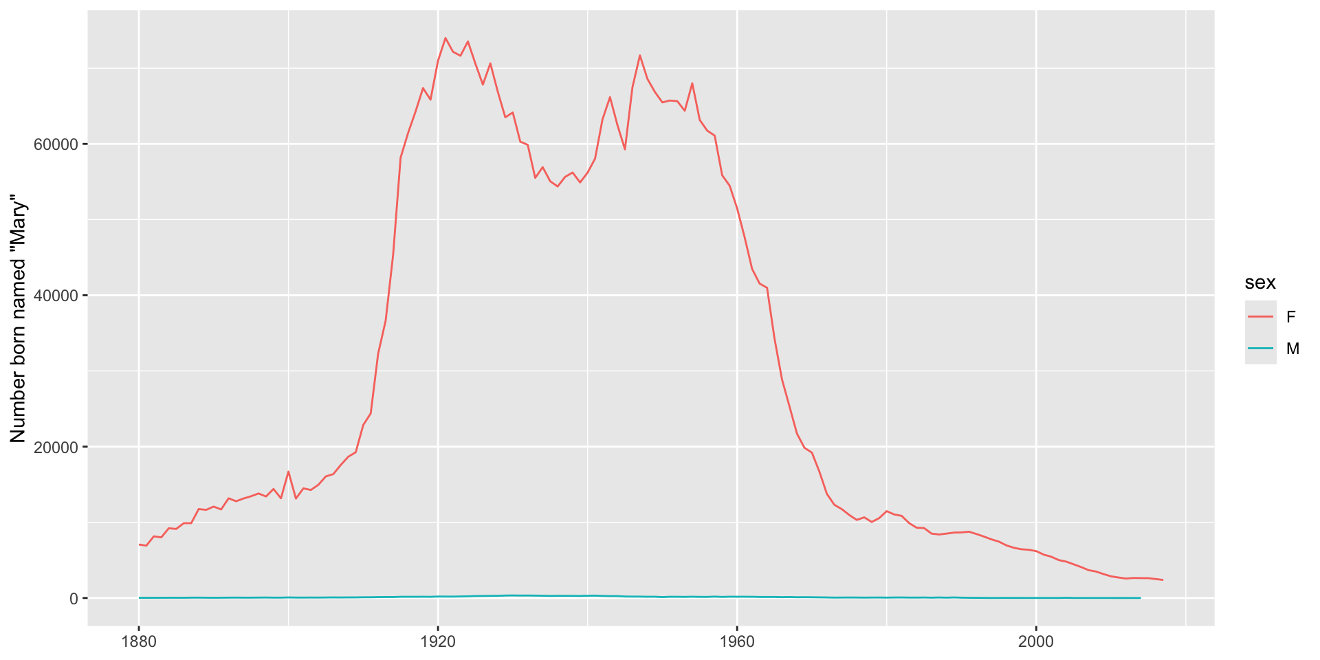
How popular has the name “Mary” been over the years?

Expand for code

babynames %>% 
  filter(name == "Mary") %>% 
  mutate(perc = prop * 100) %>% 
  ggplot(aes(x = year, y = perc)) +
  geom_line(aes(color = sex)) +
  labs(x = NULL, y = "Percentage born named \"Mary\"")

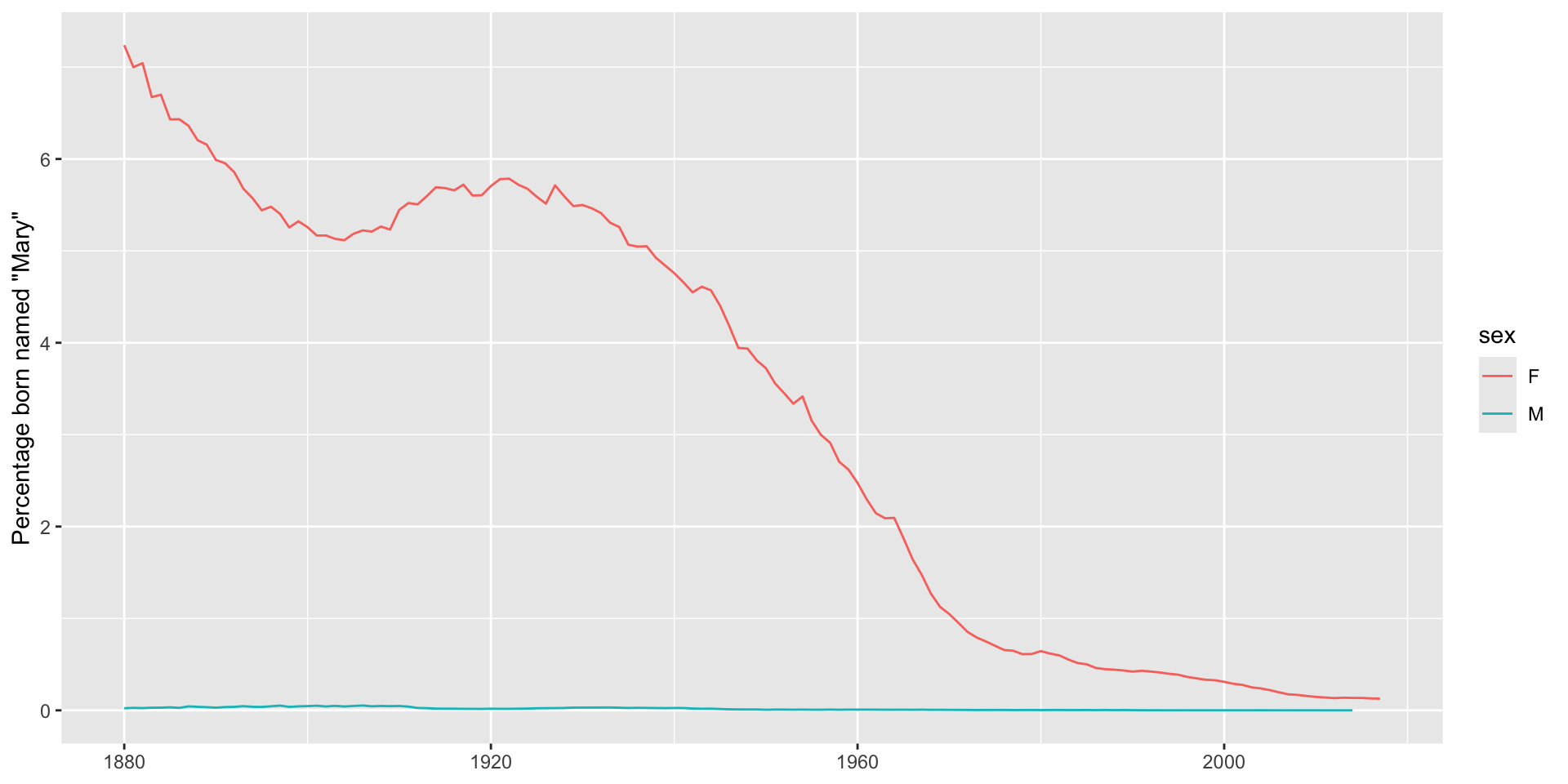
Number vs. Percentage

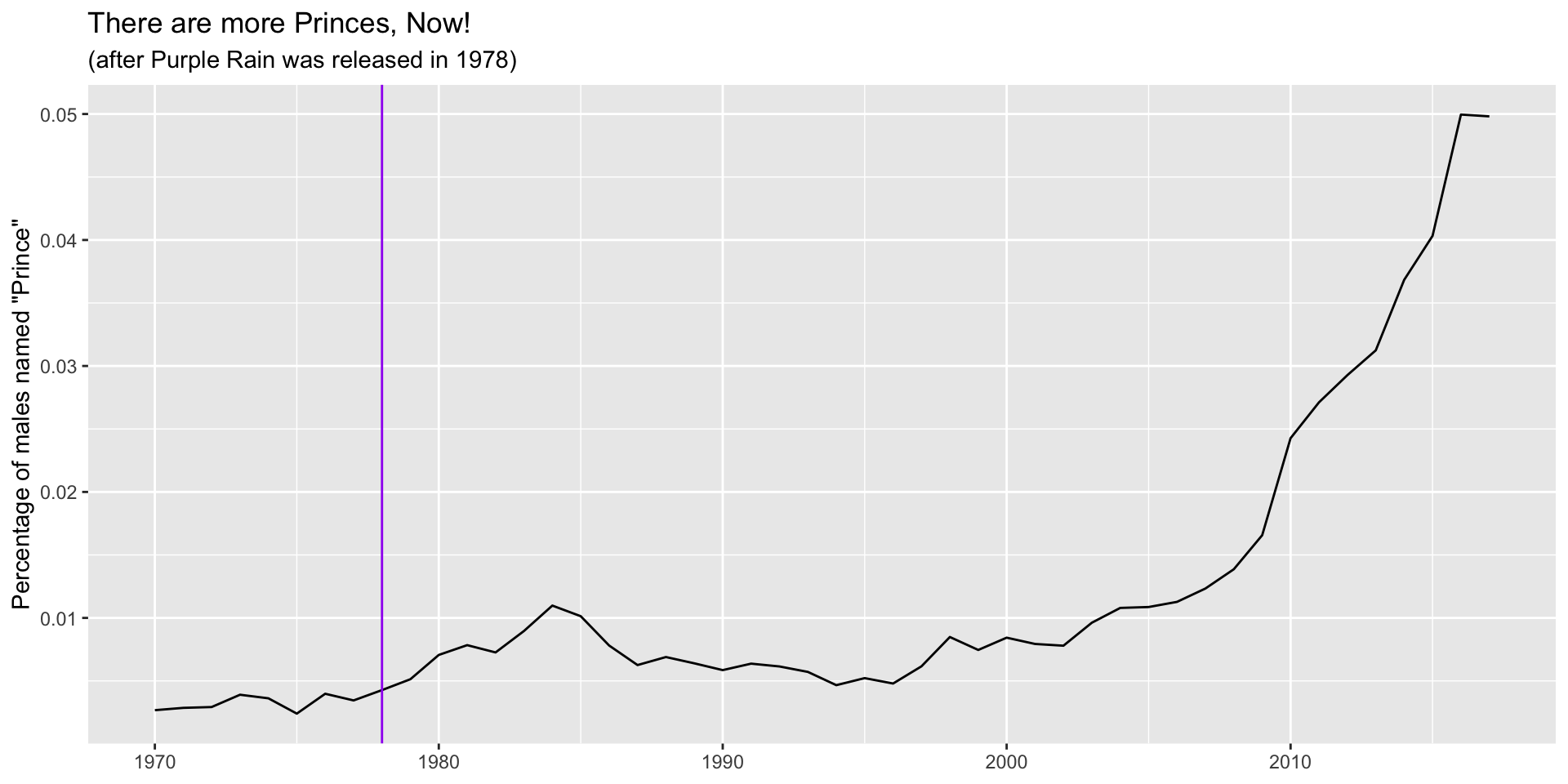
Expand for code

babynames %>% 
  filter(name == "Mary") %>% 
  ggplot(aes(x = year, y = n)) +
  geom_line(aes(color = sex)) +
  labs(x = NULL, y = "Number born named \"Mary\"")

Practice

How popular has your name been, over the years?

(Work with percentages, not absolute number of births.)

Marking a Date

Popularity of Prince

Let’s investigate the popularity of the name “Prince” as a name for boys, since the year 1970.

We will make special note of 1978, the year that Prince released his classic album Purple Rain.

Expand for code

babynames %>% 
  filter(name == "Prince" & year >= 1970 & sex == "M") %>% 
  mutate(perc = prop * 100) %>% 
  ggplot(aes(x = year, y = perc)) +
  geom_line() +
  geom_vline(aes(xintercept = 1978), color = "purple") +
  labs(
    x = NULL,
    y = 'Percentage of males named "Prince"',
    title = "There are more Princes, Now!",
    subtitle = "(after Purple Rain was released in 1978)"
  )

Two or More Names

Head-to-Head Matchup

Which name for males has been more popular over the years: “Homer”, or “Jalen”?

Expand for code

babynames %>% 
  filter(sex == "M" & name %in% c("Homer", "Jalen")) %>% 
  mutate(perc = prop * 100) %>% 
  ggplot(aes(x = year, y = perc)) +
  geom_line(aes(color = name)) +
  labs(x = NULL, y = "Percentage")

Some Ranking

Popular Female Names, by Decade

What are the top 5 most popular female names for each decade from the 1950s through the 2000-oughts?

tops <-
  babynames %>% 
  filter(year >= 1950 & year <= 2009 & sex == "F") %>% 
  mutate(decade = paste(
    floor(year / 10),
    "0s", sep = ""
    )
  ) %>% 
  group_by(decade, name) %>% 
  summarize(total = sum(n)) %>% 
  top_n(5, wt = total) %>% 
  arrange(decade, desc(total))

DT::datatable(tops, options = list(pageLength = 5))

What If …

… you reversed the order of grouping?

bad_tops <-
  babynames %>% 
  filter(year >= 1950 & year <= 2009 & sex == "F") %>% 
  mutate(decade = paste(
    floor(year / 10),
    "0s", sep = ""
    )
  ) %>% 
  group_by(name, decade) %>% 
  summarize(total = sum(n)) %>% 
  top_n(5, wt = total) %>% 
  arrange(decade, desc(total))