Confidence Intervals

Lesson 20

Packages

Make sure these are attached:

library(LSTbook)

Confidence Intervals for Parameters

Hill-Racing

?Hill_racing
View(Hill_racing)

How does winning time depend on distance and climb?

Model Equation

\[\text{time} = a + b_1 \times \text{distance} + b_2 \times \text{climb} + N(0,\sigma).\]

Confidence Intervals

time_mod <-
  Hill_racing |> 
  model_train(time ~ distance + climb)
time_mod |> 
  conf_interval()

# A tibble: 3 × 4
  term           .lwr   .coef    .upr
  <chr>         <dbl>   <dbl>   <dbl>
1 (Intercept) -533.   -470.   -407.  
2 distance     246.    254.    261.  
3 climb          2.49    2.61    2.73

These are 95%-confidence intervals for their respective parameters.

How are they made?

Model Summary

time_mod |> 
  regression_summary()

# A tibble: 3 × 5
  term        estimate std.error statistic   p.value
  <chr>          <dbl>     <dbl>     <dbl>     <dbl>
1 (Intercept)  -470.     32.4        -14.5 9.92e- 46
2 distance      254.      3.78        67.1 0        
3 climb           2.61    0.0594      43.9 4.08e-304

std.error is an attempt to estimate the standard deviation of the parameter-estimate.
It measures the amount by which the estimate could easily differ from the value of the unknown parameter.

For Example …

# A tibble: 1 × 5
  term     estimate std.error statistic p.value
  <chr>       <dbl>     <dbl>     <dbl>   <dbl>
1 distance     254.      3.78      67.1       0

We estimate that for each additional kilometer, the mean winning time increases by 253.8 seconds.
But this estimate could easily by off from the unknown parameter \(b_1\) by 3.78 sec/km or so.

Comparison

# A tibble: 1 × 4
  term      .lwr .coef  .upr
  <chr>    <dbl> <dbl> <dbl>
1 distance  246.  254.  261.

Compare with:

253.8083 - 2 * 3.784332

[1] 246.2396

253.8083 + 2 * 3.784332

[1] 261.377

Interpretation

We say:

We are 95%-confident that the mean increase in winning time associated with an additional kilometer of ditance is somewhere between 246 and 261 seconds per kilomter.

95%-Confident

What does it mean that we are 95%-confident? It means that:

The interval was computed by a formula designed so that in repeated sampling the interval produced would cover the true value of the parameter 95% of the time.

Verify This with Simulation

Imagine that the real-world data-generating process works like this:

Try It Out

Try this a few times:

The true value of \(b_1\) is 254. Usually the confidence interval contains this value.

Sample Many Times

Compute Coverage-Percentage

Making Decisions With Confidence Intervals

Is it Plausible …

… that the mean increase in winning time for each additional kilometer is less than 240 seconds?

Well, …

… the 95%-confidence interval for \(b_1\) is:

time_mod |> 
  conf_interval() |> 
  filter(term == "distance")

# A tibble: 1 × 4
  term      .lwr .coef  .upr
  <chr>    <dbl> <dbl> <dbl>
1 distance  246.  254.  261.

240 lies below that interval. So, based on the data we have, it’s not plausible that \(b_1\) could be that low.

Is it Plausible …

… that the mean increase in winning time for each additional kilometer is less than 250 seconds?

Well, …

… the 95%-confidence interval for \(b_1\) is:

time_mod |> 
  conf_interval() |> 
  filter(term == "distance")

# A tibble: 1 × 4
  term      .lwr .coef  .upr
  <chr>    <dbl> <dbl> <dbl>
1 distance  246.  254.  261.

250 lies within that interval. So, based on the data we have, it’s plausible that \(b_1\) could be that low.

Is it Plauasible …

… that the mean increase in winning time for each additional meter of climb is more than 3 seconds?

Well, …

… the 95%-confidence interval for \(b_2\) is:

time_mod |> 
  conf_interval() |> 
  filter(term == "climb")

# A tibble: 1 × 4
  term   .lwr .coef  .upr
  <chr> <dbl> <dbl> <dbl>
1 climb  2.49  2.61  2.73

3 lies above that interval. So, based on the data we have, it’s not plausible that \(b_2\) could be that high.

Is it Plauasible …

… that the mean increase in winning time for each additional meter of climb is more than 2.6 seconds?

Well, …

… the 95%-confidence interval for \(b_2\) is:

time_mod |> 
  conf_interval() |> 
  filter(term == "climb")

# A tibble: 1 × 4
  term   .lwr .coef  .upr
  <chr> <dbl> <dbl> <dbl>
1 climb  2.49  2.61  2.73

2.6 lies within that interval. So, based on the data we have, it’s plausible that \(b_2\) could be that high.

Confidence Intervals By Resampling

A Model Assumption

\[\text{time} = a + b_1 \times \text{distance} + b_2 \times \text{climb} + N(0,\sigma).\]

It was assumed that the noise is normally distributed, with a fixed standard deviation, no matter what the distance and climb are.

Residuals

A residual is the difference between the fitted value for the y-variable and the actual y-value in the data.

The trained model chooses its coefficients so that the sum of the squares of the residuals is as small as possible.

Finding the Residuals

Code

time_mod |> 
  model_eval(data = Hill_racing) |> 
  DT::datatable()

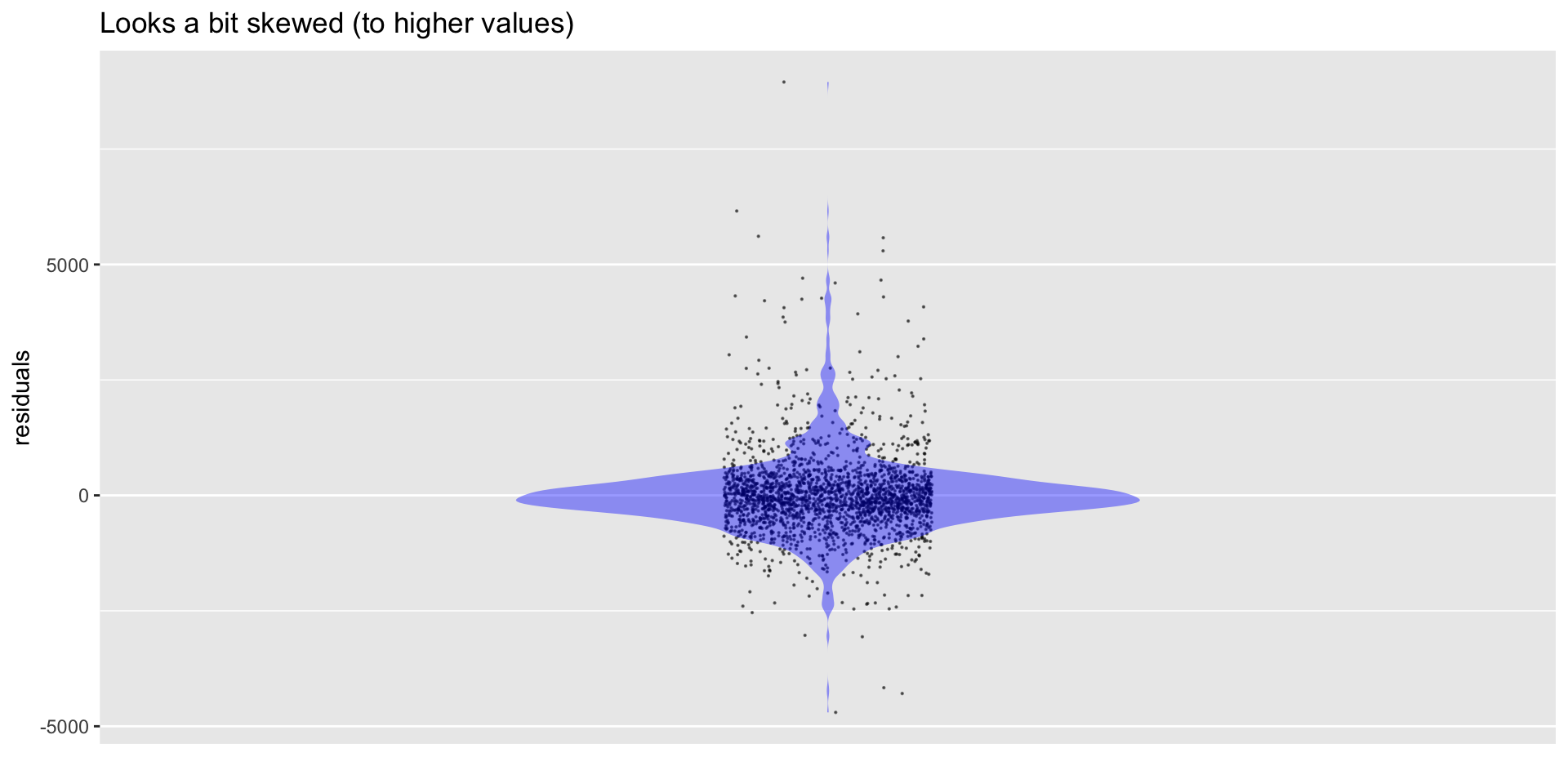
Plot the Residuals

Code

time_mod |> 
  model_eval(data = Hill_racing) |> 
  point_plot(.resid ~ 1, size = 0.1, annot = "violin") |> 
  add_plot_labels(
    y = "residuals",
    title = "Looks a bit skewed (to higher values)"
  )

Plot Residuals vs. Fitted Values

Code

time_mod |> 
  model_eval(data = Hill_racing) |> 
  point_plot(.resid ~ .output, size = 0.2, point_ink = 0.1) |> 
  add_plot_labels(
    y = "residuals",
    x = "fitted values",
    title = "Definitely a trumpet-shape!"
  )

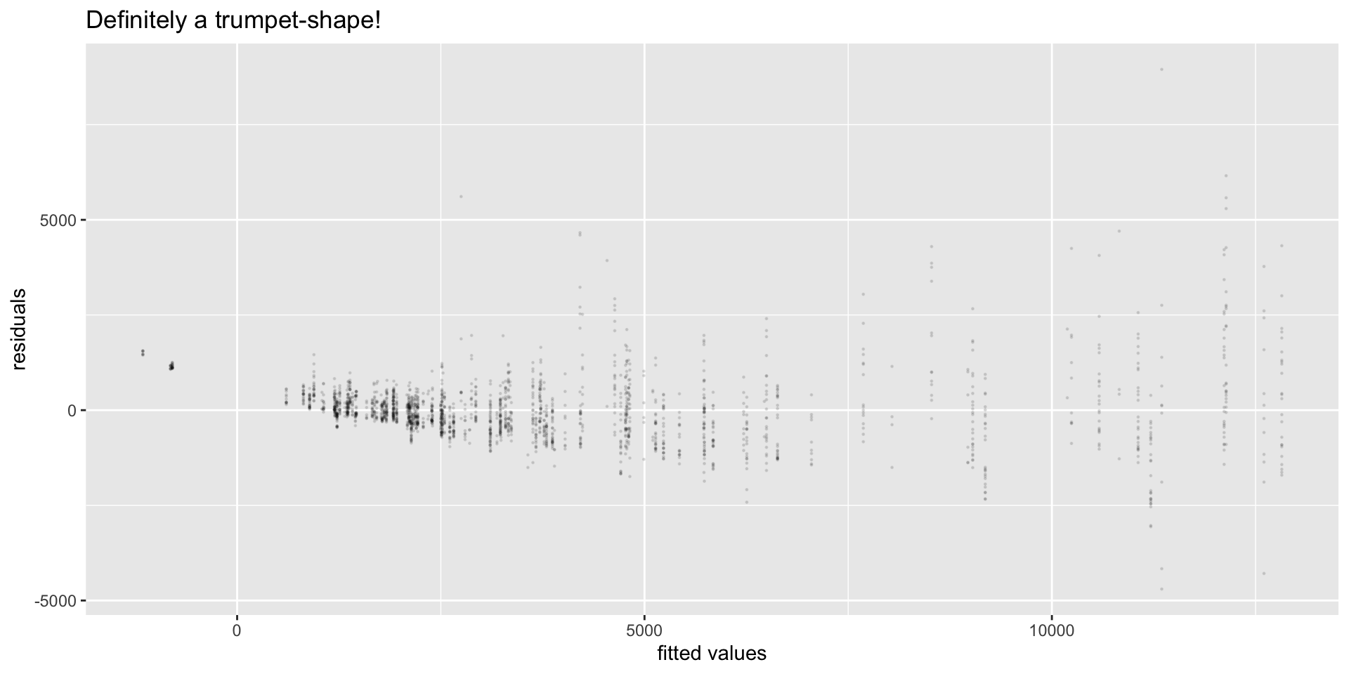
The Model Assumption …

… that the noise is normally distributed, with a fixed standard deviation, no matter what the distance and climb are …

might not be realistic!

Resampling: a Robust Method

When we cannot trust the model assumptions, we can try to make a confidence interval by resampling.

Resample

Get Percentiles

Compare with the normal-noise-based interval:

# A tibble: 1 × 4
  term      .lwr .coef  .upr
  <chr>    <dbl> <dbl> <dbl>
1 distance  246.  254.  261.

This procedure …

… is called the “percentile” bootstrap.